Control Theory - Supplemental - Vertical Arm

Introduction

For context, this post came about when one of our students asked for info on tuning the other main type of system in FRC - one where a motor powers a mechanism, and the desired position is the setpoint.

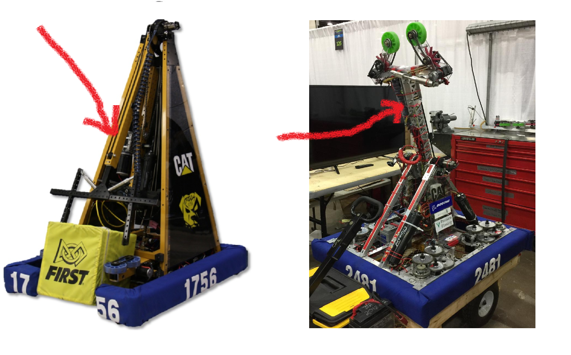
A common example is an arm on the top of a robot. For our arm, we’ll assume it’s vertical - that is to say, it lifts things from floor height to some higher elevation - Think like the 2018 game robots:

Our desired input (or setpoint) will come in terms of degrees above or below the horizon, rather than rotational velocity. As we’ll see, this leads to a different tuning methodology, but the underlying PID concept still works.

This post will come in two parts. First we’ll discuss the meaning of a “good” PID tune, relevant to any PID system you are tuning. Then, we’ll go into the specifics of tuning our vertical arm.

Defining “Good” to Get Good

We’ve thrown out a bit of terminology already related to how you judge how “good” your PID tune is.

Like any good exercise in engineering, there’s terminology which refers to specific measurements of goodness. Let’s take a quick step back to formalize what these actually are.

Keeping with our examples so far, we’ll frame all of our discussion in terms of the time domain step response of our system.

All that follows in this section is just terminology - specific words control systems engineers to describe physical behavior in a way that communicates meaning to others.

Then again, keep in mind - terminology is important! On some grand scale of “importance” - understanding the underlying concept is probably more important, but immediately following that is the ability to communicate it to others.

\soapbox.

General System Response Classifications

When tuning a system and looking at its step response, there are fundamentally three categories of system response. Systems are said to be Overdamped, Underdamped, or Unstable.

An overdamped system will slowly approach the desired value, hopefully settling out just barely underneath the desired value. It’s generally pretty gradual, and has no oscillation, and never crosses or goes above the desired value.

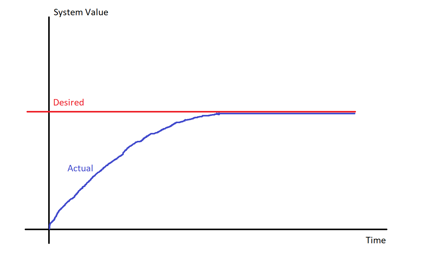
The name should make sense - if you think of friction or stiffness in the system as a “damping” force, an overdamped system has quite a bit of damping. Sometimes this is desired, sometimes it is not (as we’ll discuss later). But for now, just remember the association of the word with the meaning.

Similarly, an underdamped system will have much less damping. In these systems, the actual value overshoots the desired value, crossing and turning around multiple times before settling down. An underdamped system will always have some amount of oscillation.

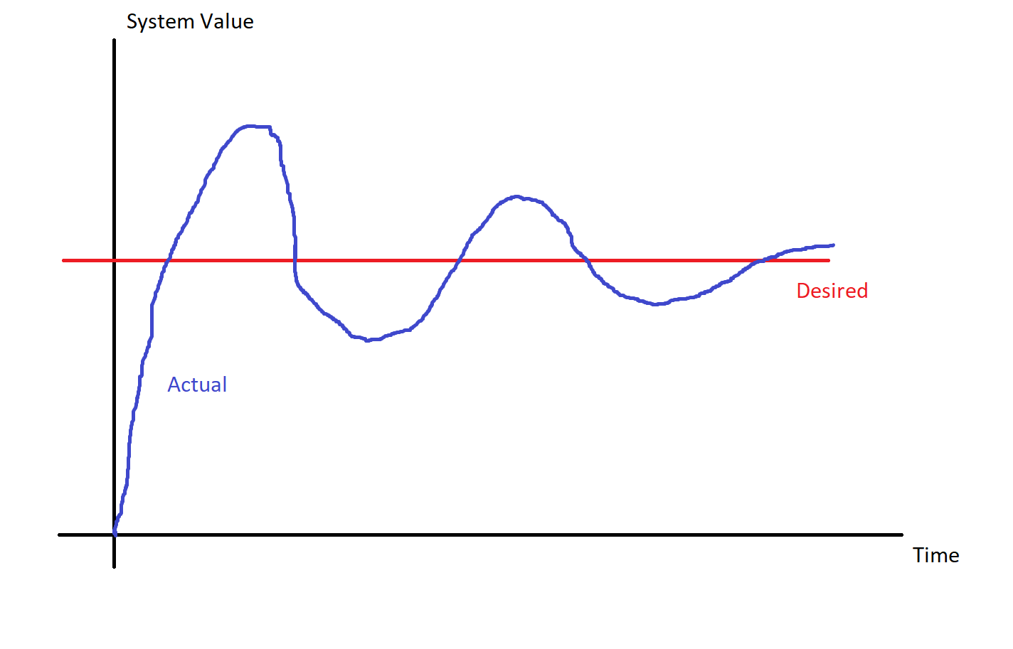
For systems that involve a PID controller, the P gain tends to be the “knob” that pushes a system between overdamped and underdamped. Additionally, the D gain can take a system with underdamped characteristics, and make it look more overdamped.

Both of these system types are stable - this means that as time progresses, the actual value converges toward the desired value. It’s also very possible that you might get a system which is unstable - where the actual value doesn’t actually go toward the desired value. These often come in one of two flavors.

The first flavor is the “it blows up from getting too big”:

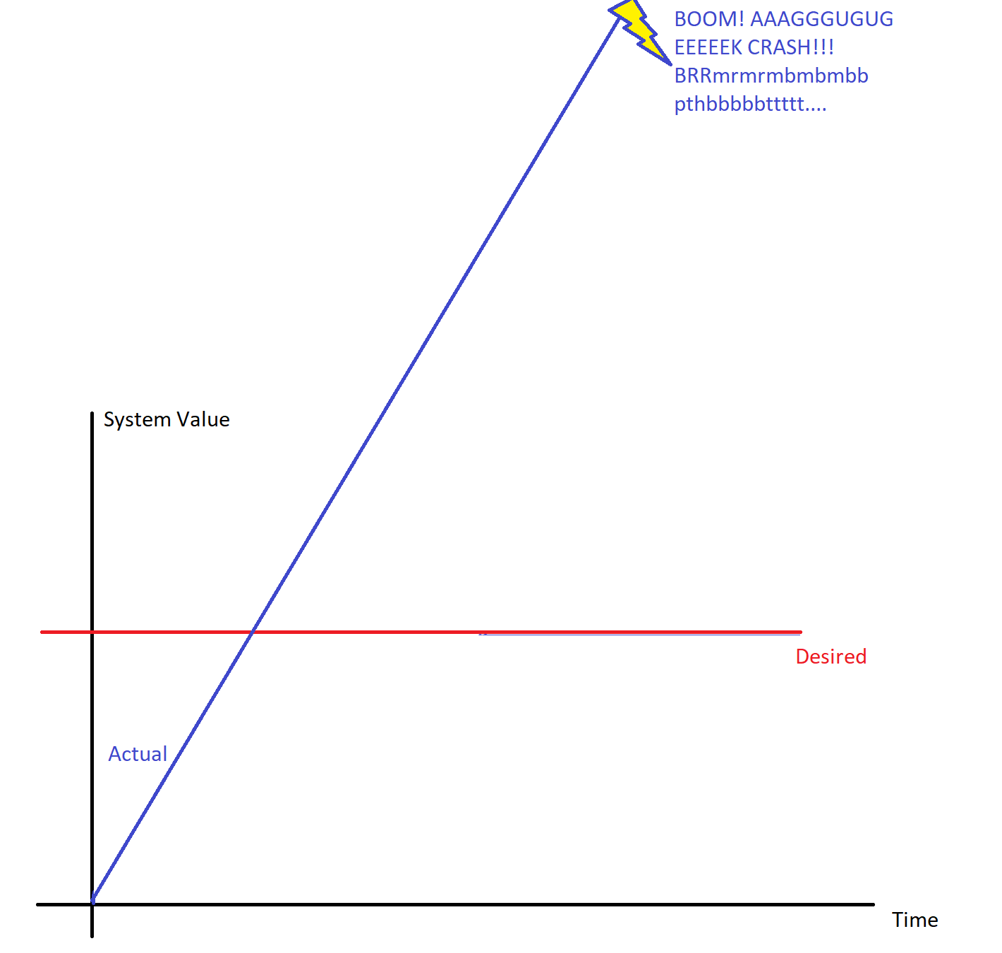
Here, for whatever reason, the system’s value just shoots off in one direction, never really going where we want it. In general, in cases like this, you’ll hit some mechanical or electrical limit, break something or let the magic smoke out, and have some other subteams angry at you. Definitely not recommended.

The other flavor of unstable stays somewhat close to the desired value, but never “settles down”.

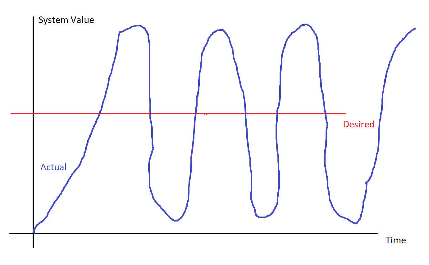
At best, this will be a robot that looks really bad and uncontrollable, which means you don’t get picked in elimination rounds. More often, the motion causes parts to wear out prematurely and also break. Again, bad news bears. Also not recommended.

Taking these examples: part of the definition of “good” usually involves:

1. System should be stable
2. System ought to be slightly overdamped or slightly underdamped (depends on the situation). Having the other is less than desireable.

Quantitative Goodness Measurements

Aside from the above qualitative system classification, for stable systems, we also commonly define a few measurements of system response.

Rise Time & Settling Time

There are two main time-based measurements for talking about your system response.

Rise time refers to the duration between when the desired command changes, and the first time the actual value gets to the desired value.

Settling time refers to the duration between when the desired command changes, and when the actual values settles down within some acceptable error from the desired value.

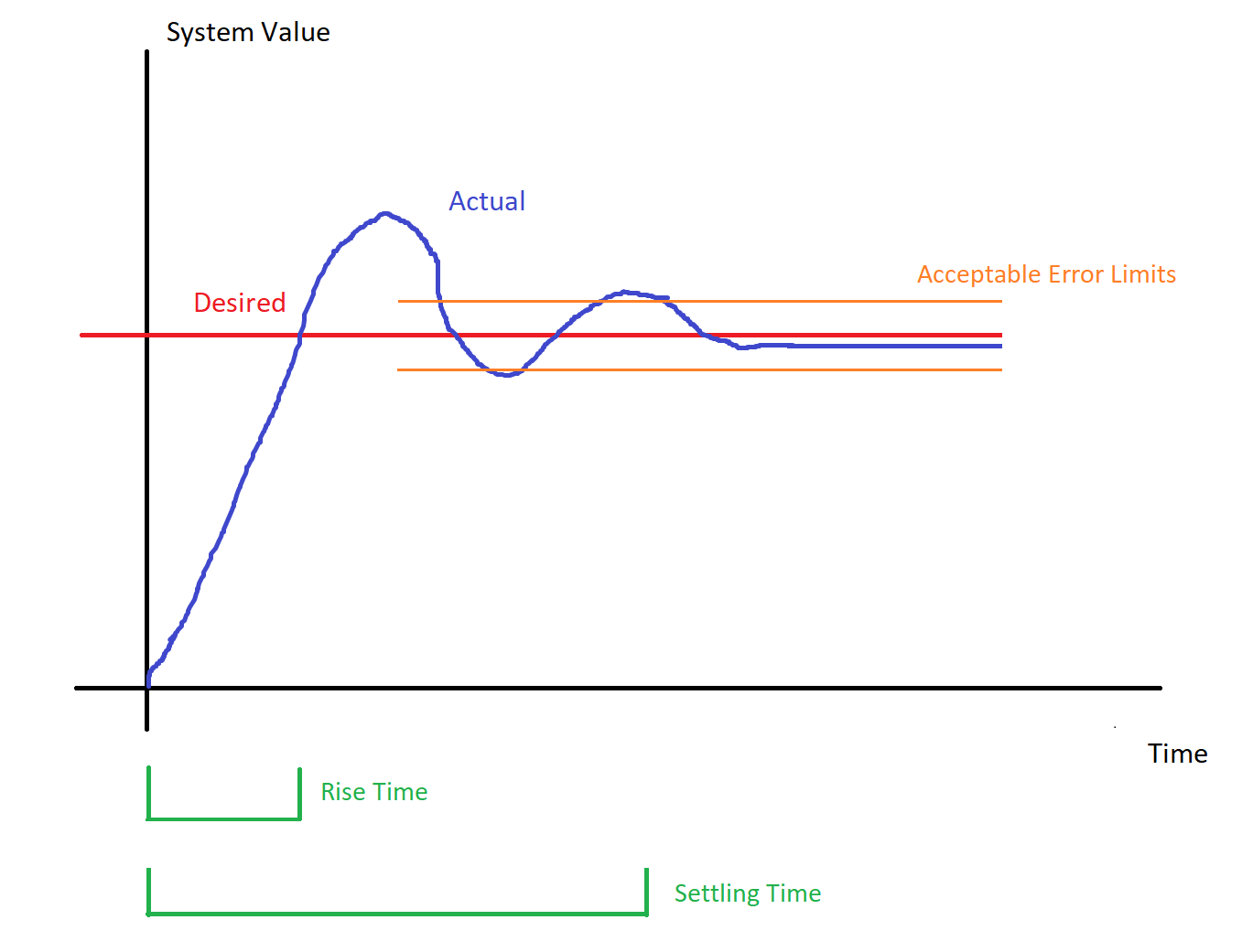
Overdamped systems will have a longer rise time than underdamped systems. Settling times can vary quite a bit, depending on system dynamics.

In general, more powerful motors, less mass, and more P gain all help you achieve better rise time.

In general, more powerful controllers with faster feedback systems and less delay help you reduce your settling time. More mass can help your system “dampen” itself out mechanically. More D gain can increase damping to a point, but will also eventually cause instability. Less mass can allow your controller’s D term to do damping more efficiently.

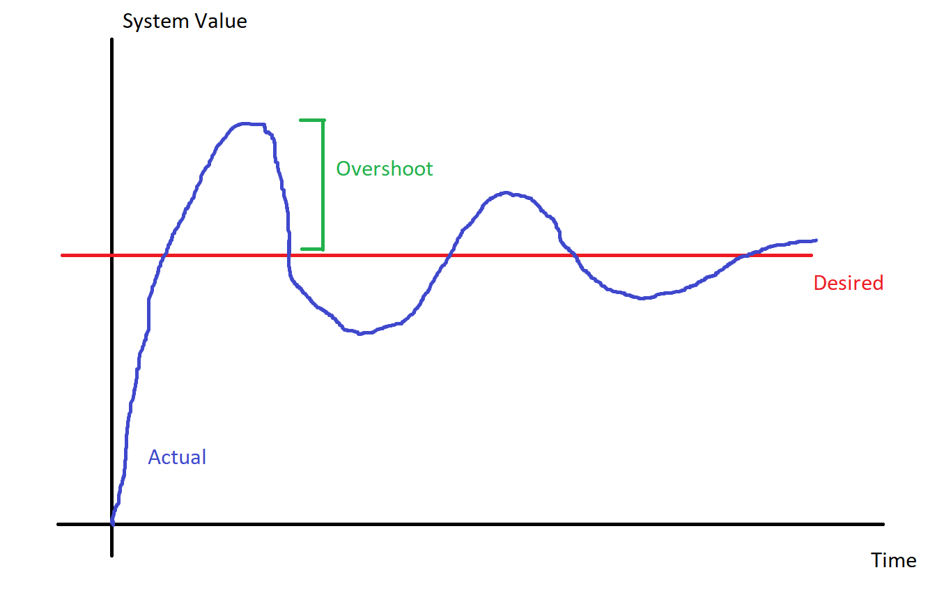
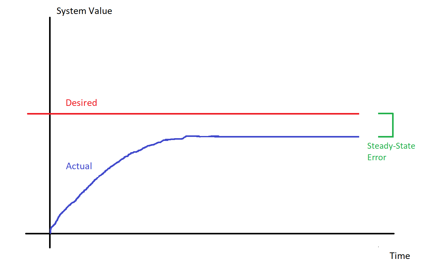
Overshoot & Steady State Error

There are also two value-based metrics for talking about your system response.

Overshoot refers to how much the actual value goes past the desired value before coming back toward it.

Steady State Error refers to how far off the actual value is from the desired value after all transient behavior has died down, and the system is fully stabilized.

In general, decreasing P and increasing D will lower the amount of overshoot you have. Increasing the physical mass or increasing the friction of the system can also do the same thing.

In general, increasing P and increasing I will decrease the amount of steady state error you have. Decreasing the mass of the system or decreasing the friction will allow I and P to do their jobs more effectively.

Tune, but Don’t Discount Mechanical Changes

Note that if you have multiple “problems” with your tune system, you may have some conflicting requirements. For example, if your overshoot AND your steady state error are both too big, you’ll have a hard time adjusting P (as changing it makes one issue better, while making the issue worse.)

It’s important to try to get your PID gains dialed in as much as you can, but also keep in mind that some systems are really hard to control. You may hit a point where you can’t get it any better by adjusting gains alone, and need to think more creatively. Some of these “more creative” changes include:

1. Adjusting the mass of the system (adding or removing weight from the actuated mechanism)
2. Adjusting the friction of the system (using grease or dashpots)
3. Changing gearbox ratios
4. Adding motors to the system
5. Adding springs or counterweights at strategic locations to add additional force
6. Increasing the quality of the PIDF controller system (ie, move from RIO-implemented controller (~100Hz) to onboard Talon SRX or Victor SPX (~1000Hz) controllers.)

The “rule of thumb” I tend to tell my team - If it’s impossible to control manually, with a thrifty throttle and a human watching it, it will be very hard to control with software. It’s definitely not an axiom, but gives mechanical and electrical teams a “stick in the mud” to understand if the thing they’ve created is anywhere in the realm of controllable.

Choosing Criteria

How does one pick from amongst these criteria for their specific situation? Unfortunately, it just depends. Thankfully, it’s often intuitive, or can be derived from robot design discussions. How accurate does manipulator XYZ have to be? How quickly does it need to get into position for us to meet our cycle times (and no, “fast as possible” isn’t a detailed enough answer :D ).

In general, you’ll want small rise & settling times, minimal overshoot and no steady-state error. However, as you have seen (or will see), it’s hard to get all of these at once. Usually, achieving one will be more important than the others.

For example, consider if you were controlling the temperature in your house. The temperature is currently 50 degrees F (brrrrr!!!), and you want it to be 70 degrees F. You want the temperature to get to 70 quickly, but not so quickly that it overshoots the 70 degree mark, and shoots up to 100 degrees before settling back down. That would be a waste of energy, and a longer time of you being uncomfortable. An underdamped controller is generally desired in cases like this, with enough I gain to cancel out steady-state errors.

In contrast, take our shooter wheel example from last time. Generally, you’ll want to spin the wheel up to a stable launch speed as quickly as possible (assuming this is a component in your robot’s overall cycle time). This means aggressive P - a bit of overshoot isn’t horrible, nor is a few RPM of steady state error.

Finally, the example we’re about to see - consider if you are controlling the angular position of an arm - accurate positioning of the end of the arm (within fractions of a degree) is probably desired. Speed is important, but not at the cost of getting the gamepiece at the wrong place. Overshoot may also be a concern, as the arm has physical limits of travel - too much overshoot may be mechanically damaging.

In conclusion, the requirements for what constitutes a “good” PID tune are derived from your requirements for what makes a good robot. Which, of course, depends on your robot, and the year’s game. It all just depends.

What “In General” Means

One final note (I promise). I’ve used the weasel-word phrase “in general” a lot. Here, I mean it to imply “for most of the FRC-encountered situations”.

Software bugs, weird mechanisms, measurement delay, very-sensitive systems, and a whole host of other things can make the assumptions laid out here invalid. For that reason, it’s very hard for me to ever say “Always”.

Keep this in mind while tuning. These things do work. They’re out in the world everywhere. If you’re struggling to make it work in your situation, there has to be a reason why. Maybe it’s because you have a software bug. Maybe it’s because the physical manipulator is very exotic.

The best I can tell you - approach the problem systematically.

Verify the assumptions of your software - have proof it operates as you expect.

Compare your design to those used successfully by other teams. Where are they the same, and where are they different? Do those differences matter? Do the math to prove it!

Finally, pull in subject-matter experts - mentors, industry professionals, more experienced students, chiefdelphi, or even myself (see the email at the bottom).

Arm System Model

On to the actual arm!

Basic Description

Ya ever heard of chicken on a stick? Well, we’re gonna model the arm as mass on a stick. Just some weight (from a claw or intake motors or similar), suspended on the end of a long, thin rod (which weighs relatively little).

The arm is constrained to rotate through just one plane, going up and down powered by a motor at the “shoulder”. The motor is of course run through a (fairly-high reduction) gearbox. When you run the motor in one direction, the arm goes up. In the other direction, it goes down.

Additionally, our arm will be vertical - the plane it travels within is parallel to the direction gravity pulls on the arm. This means that when the arm is stretched “straight out” in front of the robot, gravity will be pulling it down toward the ground.

Mathematical Description

Since this is a bit abbreviated, I won’t go through the full derivation of this system. However, it’s not too bad to build up an equation from the bits and pieces we already have.

To do so, we’ll use the shoulder joint of the arm as our origin and reference point. All torques, speeds, accelerations, and angular positions will be measured about this point. Additionally, we’ll use kinda-standard angle notation, such that $0^\circ$ is pointed “straight out in front” of the robot, $90^\circ$ is straight up in the air, and $-90^\circ$ is pointed at the ground.

Overall, the acceleration of the arm is determined from the following forces acting on it:

1. $T_{m}$ - The motor (via a gearbox), which in turn in impacted by an applied voltage which we can control as we please.
2. $T_{f}$ - Friction (works against rotational motion of the arm)
3. $T_{g}$ - Gravity (pulls the arm toward the $-90^\circ$ point)

Using Newton’s second law for rotational forces, we can assemble our basic equation:

$$T_{m}(t) + T_{f}(t) + T_{g}(t) = I \alpha(t)$$

And expanding each term, we arrive at the monster:

$$\frac{N_{out}}{N_{in}} \frac{K_T}{R} \left( V_{in}(t) - \frac{N_{in}}{N_{out}} K_{V} \omega(t) \right) - K_{f} \omega(t) - m g \cos(\theta(t)) = m r^{2} \alpha(t)$$

Where:

• $\frac{N_{out}}{N_{in}}$ is the gearbox ratio
• $K_T$ is the motor torque constant
• $V_{in}(t)$ is the motor input voltage
• $K_V$ is the motor voltage constant
• $\theta(t)$, $\omega(t)$, and $\alpha(t)$ are the angular position, speed, and acceleration of the shoulder joint shaft.
• $K_{f}$ is the effective kinetic rotational friction constant of the system
• $m$ is the mass of the end-effector on the tip of the arm
• $g$ is the gravitational constant ($9.81 m/s^2$)
• $r$ is the length of the arm

Notice the minus sign on the frictional term is chosen to ensure the frictional torque opposes motion, and the gravitational torque always pushes toward $-90^\circ$.

Re-arranging to group terms, pulling constants into nice buckets, substituting continuous time $t$ for discrete samples $n$:

$$\alpha[n] = C_1 V_{in}[n] - C_2 \omega[n] - C_3 cos(\theta[n])$$

With

$$C_1 = \frac{N_{out} K_T}{mr^2N_{in}R}$$ $$C_2 = \frac{K_T K_V}{mr^2R} + \frac{K_f}{mr^2}$$ $$C_3 = \frac{g}{r^2}$$

Since acceleration is the derivative of velocity, we can approximate $\alpha[n]$ in terms of $\omega[n]$:

$$\alpha[n] = \frac{\omega[n] - \omega[n-1]}{T_s}$$

And similarly, since velocity is the derivative of position, we can approximate $\omega[n]$ in terms of $\theta[n]$

$$\omega[n] = \frac{\theta[n] - \theta[n-1]}{T_s}$$

Math sticklers, avert your eyes for a paragraph.

If you were to substitute these into our equation, you’d end up with an equation that stinks to solve symbolically for $\theta[n]$, because $\theta[n]$ appears both inside and outside a $\cos()$ function. Maybe there’s a good way to solve it. I don’t know offhand. What I do know is I can cheat a bit and use some one-sample-delayed assumptions that, for sufficiently small $T_s$, make our equation much more workable. There’s enough sensor delay in our feedback (relative to $T_s$) that I honestly don’t think it will mess up the solution too much. I think. Let’s just go with it, Wild West style. Shoot math from the hip. That’s how we roll. I guess. Remember, all models are wrong.

Ok, math people, come back, and don’t try to check my work.

The final equation for position, in terms of things we know already or can control, is:

$$\theta[n] = \frac{T_s^2 C_1 V_{in}[n] - T_s^2 C_3 \cos(\theta[n-1]) + \theta[n-1]\left( T_s C_2 + 2 \right) - \theta[n-2]}{T_s C_2 + 1}$$

If that doesn’t make my eyes ooze out of their sockets, I don’t know what will.

Step Response

We’re definitely going to want to play around with this guy to get some intuition for how it works. We’ve got another sidebar with our system behavior in it.

Since that equation is ever so intuitive, let’s see what happens when we put our arm at horizontal, then let the system rip with some constant voltage applied.

Start by moving this slider to zero volts - no motor command at all. You should notice the arm fall down to the $-90^\circ$ position and stay there. It swings back and forth a bit till friction stops it.

This should totally make sense - in this configuration, the arm is like a pendulum. Pendulums oscillate due to the pull of gravity.

Try bumping up the voltage by a volt or two. You should also see something logical - the motor causes the arm to settle out at some position “higher up” than before, as the motor fights gravity.

Eventually if you give enough voltage, your arm can swing all the way around in a circle. Wheeee! This is what, in my business, we call unstable.

Simply applying a constant voltage doesn’t work all that well at getting the arm to a desired position. Clearly, for any position, our controller will have to find that nice happy voltage at which the arm maintains the proper position. It may also have to adjust the voltage a bit higher at first to get it to the setpoint.

Controller Setup

We’re gonna cut straight to using PID this time. But no F. F isn’t exactly useful, or not as we used it while doing the shooter wheel exercises. The motor command required isn’t exactly proportional to the angle (think, for example, 0 degrees - definitely more than zero motor command required to keep the arm there). We’ll wrap back to this later, but for now we’ll skip F.

First Pass at Tuning

Just as before, use the same doubling/halving technique to get close, then tweak once close.

Start by tuning P, just to where oscillations around the setpoint start to happen.

First do the big adjustments:

Then do smaller tweaks when you get closer:

Or, if you get completely lost, start over:

Hint: 65.0 is a good value for P

Then tune D to get rid of the oscillations:

Big adjustments:

Small Tweaks:

Start Over:

Hint: 6.87 is a good value for D

Finally, you’ll notice we do have some steady state error. Tune I to get rid of that:

Big adjustments:

Small Tweaks:

Start Over:

Hint: 13.1 is a good value for I

Varying the Setpoint

As before, we’ll want to vary the setpoint to ensure our controller can achieve a range of outputs equally well.

As you move the setpoint around, even with well-chosen PID gains, you’ll notice the overshoot and oscillation vary quite a bit, depending on the setpoint. More simply, the gains chosen do not work equally well across all setpoints.

This should be expected. Our system is non-linear (due to the presence of the $\cos(\theta[n-1])$ term), but the PID algorithm is fundamentally designed to work around linear systems. It can get close, but it’s honestly not the best answer in this case.

What to do? One option is to pick the point at which you want to hold the arm, and keep it there. You pick PID gains that work well for $\theta_{des}$, and ignore other values. Especially if your arm has a very limited range of motion, or always goes between the same two points, this isn’t a bad option at all.

Another method is to add a (slightly) complex feed-forward term into our PID controller to compensate for the nonlinearity. This is what we will attempt to do now.

Removing Non-Linearity

Since we know our system, we can use a more complex F term to remove the nonlinearity. We get clever to eliminate gravity.

The key fact: Gravity is proportional to $cos(\theta_{act}(t))$. So, we will make an F term which is also proportional to $cos(\theta_{act}(t))$. When properly tuned, we will effectively cancel-out the effects of gravity on the system.

We will modify our PID equation to add the extra term:

$$v_{PID}(t) = K_{P} \theta_{err}(t) + K_{I} \int_{x=0}^{x=t}\theta_{err}(x)dx + K_{D} \frac{d\theta_{err}}{dt} + K_{F} \cos(\theta_{act}(t))$$

As a quick note on software - this technique is usually referred to as “arbitrary feed-forward”, and is supported by both the Talon SRX and Spark MAX speed controllers.

Re-tuning

Need to start again, because all our gains no longer should be accounting for gravity.

Now, we’ll start tuning with F.

F can be calculated as the voltage required to hold the arm level (easy to empirically determine on a robot).

Since our arm starts at 0 degrees anyway (at least in this simulation), you’ll want to just keep bumping F up until the arm stays at zero degrees, even with all feedback (P, I, D) gains at zero. Note that on this system, F gets really sensitive around this point - the bump ups and downs will be quite small.

Again, the goal is to start the arm at 0 degrees, and tweak F until the arm holds its position at zero degrees (not the setpoint).

Use the double/half/tweak methodology first.

Then do smaller tweaks when you get closer. This will take a lot of clicking.

Or, if you get completely lost, start over:

Hint: 5.91 is a good value for F

Next we’ll move back to tuning P, again just to where oscillations start to happen. As we move P away from zero, the arm will now start to move toward the setpoint.

First do the big adjustments:

Then do smaller tweaks when you get closer:

Or, if you get completely lost, start over:

Hint: 32.76 is a good value for P

Then tune D to get rid of the oscillations:

Big adjustments:

Small Tweaks:

Start Over:

Hint: 3.27 is a good value for D

Finally, there may be a bit of steady state error left. If so, tune I to get rid of that:

Big adjustments:

Small Tweaks:

Start Over:

Hint: 0.0 is a good value for I, at least as I tuned it.

And, again, try varying the setpoint across the range of angles desired:

This time, you should observe much less variance in overshoot and convergence time across the range of possible setpoints. In general, your arm should be working much much better now.

We Just Did Plant Model Inversion

It should be noted that our “arbitrary feed forward” term we used here is a simplified form of plant model inversion. It’s actually the same as the shooter wheel’s feed forward as well for steady state. The basic idea behind all of it is that if you can get a mathematical description of how your plant model works, you can inject the inverse of that knowledge into your controller to help account for the system dynamics that a plain old PID controller doesn’t need.

With knowledge of these plant dynamics, the only thing left for the PID closed-loop portion to do is compensate for transient, external loads, or any behavior not accounted for in the inverted plant model. This is nice for two reasons.

For one, it means that your plant model doesn’t have to be perfect. In fact, anything (even a constant value) is better than what you have without it (which is literally an assumption that the plant does nothing).

For two, it means the PID gains don’t have to be as big as before, having less behavior to “fight” against. This implies they can be more aggressive toward getting your manipulator to the setpoint angle.

But - all these advantages can only be achieved if you can build up a reasonable mathematical model of how your real world system works.

Conclusion

Hopefully this gives a good demonstration of how to tune PID in another common situation! Play around with these things and see what you can see. The advantage of these online simulators is the instantaneous feedback - you can clearly see what each adjustment is doing in nearly-real time. Such a luxury is harder to come by on a physical system. Plus, astable calibrations (like ones that cause the robot arm to start flying in circles) can be damaging. For this reason, doing the learning in a simulated environment is definitely a good idea. Hone your skills of tuning here, and then take them to the real world robot later.