Control Theory - PID & Controller Design

Introduction

Welcome to post 3 in our series on controls engineering. In this post, we’re going to explore the behavior of the motor model we’ve built up, try to create an intuition for how it behaves. We’ll establish a couple criteria for what we want it to do, and lead into the application of a classic PID controller.

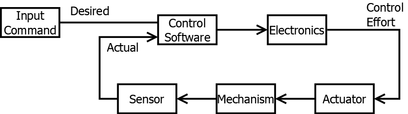
Recall our standard model of how a control system is laid out:

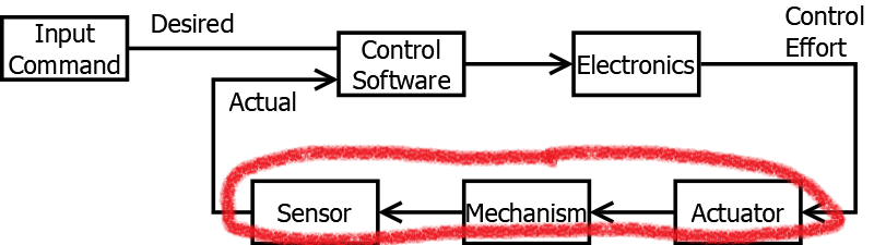
For context, in part 2, we covered what sorts of math equations go inside the plant portion of the control system:

A bit of an aside to the reader: The more I’ve been writing this series, the more I’m realizing what a disservice I’m actually doing to modern control theory. We’re using time domain analysis to build up all our understanding. Professional controls engineers, working on modern systems, don’t work in this domain. They’re using things like Linear Algebra, State-Space representations, LQR, and a whole host of things that, for better or for worse, I don’t have too much exposure to. I feel a bit bad that we’re not getting to the point where we can explain these.

You have to walk before you can run, and walking still gets you from point A to point B. What I always have to remind myself - This is just a high school robotics competition. Using LQR to design a super optimal control system is a valiant cause, one from which much can be learned. But it’s far from required for success.

The takeaway I guess I want readers to have: Enjoy our time here in the time domain space. Build up your intuition of how things evolve over time. Know that even if you get to the end of this series of posts, and learn everything they have to offer - there is still more. The pro’s can teach you much.

Plant Model Response

One of the pieces of terminology thrown around for these systems is response. It’s a generic term that simply means “Given some input, how does the output act?”.

You can describe the response to a specific input. For example, if you apply 12V to the motor, you can say the motor’s response to that 12v input is to increase speed. Response might also be more generic - if you have an equation, you might be able to describe the response to any input concisely.

When analyzing the response of a system, we generally divide the analysis into two parts: Transient and Steady-State. Transient Response refers to how the system acts immediately following some disturbance in input. If you suddenly change the input voltage to a motor, its shaft will change speed - the manner in which it ramps up or ramps down is this transient response. Separately, after the input has been stable for some time, the output usually stabilizes as well. Steady-state refers to the system behavior after all of the “transient” behavior has died down. In our motor example, if you were to adjust the input voltage from 12V to 8V, you’d see the motor slow down. The speed it settles at could be called the “Steady State” response.

To analyze system response, we generally need to expose the system to a variety of different inputs.

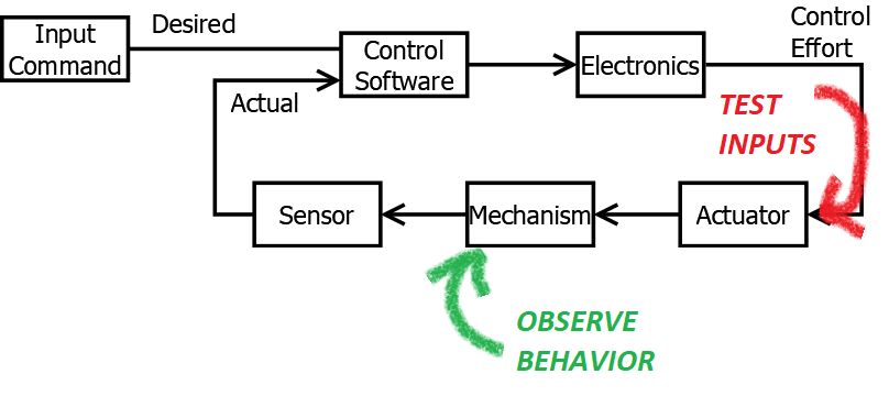
There are a few types of input that are very good to use, because you can learn a lot about the system from just a few trials (rather than shooting in the dark a lot).

The simplest is usually called a “unit step”. It’s a fancy math way to describe “flipping on a switch”. If you’re all into formal definitions, I like the piecewise definition:

$$u(x) = \begin{cases} 0 & x < 0 \\ 1 & x \geq 0 \end{cases}$$

The input to the function (here notated as $x$) is usually some function of time. You stretch and scale the function to indicate the turn-on time, and its size.

For example, if you wanted to describe “turning on” the motor (apply 12V) at time = 1 sec, you could describe the input voltage $v(t)$ with the equation

$$v(t) = 12u(t-1)$$

It should be noted that the definition of this guy doesn’t change all that much when you go from continuous $(t)$ to discrete $[n]$. The output is $0$ for all $n < 0$ and $1$ for all $n \geq 0$.

Practical Example - Shooter System Response

Let’s try to insert our function into the shooter wheel system we described last time. We’ll choose it as the function to describe how the voltage input changes over time, and see how the speed changes.

Intuition

Before we hit the math, let’s think through what we expect to happen.

• Before the voltage turns on ($t < 0$), the wheel should not be turning.
• As soon as the voltage turns on, the wheel should start spinning.
• The higher the voltage that is passed in, the faster it should be going.
• The wheel should hit some maximum “steady state” speed, and stay there.

Of course, most folks would thing this is pretty obvious. However, it’s important to keep it in mind. We can use the math equations to show our intuition to be true, or use the intuition to validate we didn’t get something wrong in the math.

Nominal Behavior

Recall the equation we derived in part 2:

$$\omega_{wheel}[n] = \frac{T_s C_1 V_{in}[n] + \omega_{wheel}[n-1]}{( 1 + T_s C_2 )}$$

Let’s see if we can get an idea for how this thing reacts when we apply an input voltage. We do this by making two assumptions:

1. We will apply 12 volts at the time 0 seconds ($t = 0$). This can be represented using our unit step function: $v[n] = 12*u[n]$
2. We will assume the wheel was stationary prior to start. This means that $\omega_{wheel}[-1] = 0$

Based on this, we can draw the following plot of wheel speed, over time:

As a side note, the $C_1$ and $C_2$ values have been chosen to represent a single 775 pro motor, through a reasonable gearbox, through a typically-sized shooter wheel. See this javascript file for more details on those assumptions.

If you stare at the graph, it certainly appears our initial suppositions are confirmed:

• For times to the left of the Y axis, we see our speed is zero.
• At $t = 0$, on the Y axis, voltage turns on, and our speed starts to increase.
• To the right of the Y axis, speed starts to increase as time goes on.
• As time goes on, we see the speed caps out at around 3500 RPM.

Extracting the Steady-state behavior.

As a brief tangent - it should be noted that you can extract these conclusions from the equation itself. Even if you don’t trust your eyes on the chart, you can still prove it logically.

For example - If we $\omega[n]$ and $V_{in}[n]$ are zero for all $n$ less than zero, we can see the equation becomes:

$$\omega_{wheel}[-5] = \frac{T_s C_1 * 0 + 0}{( 1 + T_s C_2 )} = 0$$

Additionally, if when we assume “steady-state”, we assume that $\omega_{wheel}[n] = \omega_{wheel}[n-1]$ - the mathematical way of expressing “$n$ is large enough such that $\omega_{wheel}[n]$ is no longer changing”.

In this case, we can state:

$$\omega_{wheel}[n] = \frac{T_s C_1 V_{in}[n] + \omega_{wheel}[n]}{( 1 + T_s C_2 )}$$

which simplifies to:

$$\omega_{wheel}[n] = \frac{C_1}{C_2}V_{in}[n]$$

And, again, assuming $V_{in}[n]$ is just a constant for large $n$, means that our “steady-state” $\omega_{wheel}[n]$ is in fact also a constant.

Huzzah! Isn’t math fun?

A Brief Step Back - The Goal

One key thing to remember, or learn, going forward: A consistent shooter wheel must be running at a constant, defined velocity, prior to injecting a ball. That’s right - you need to keep your rotational velocity (RPM) steady, if you want to make sure your launched ball always travels through a consistent arc. The reason for this is again based in physics - the energy imparted to the ball controls its arc, and energy imparted is related to the velocity of the shooter wheel.

Here’s the key, if you haven’t noticed yet - we have the ability to command the motor’s voltage, not it’s speed. The speed is dictated by a whole slew of additional physical parameters. Though we’ve built up this math model of how things are supposed to work, this isn’t a perfect transform we can invert to get an answer of voltage->speed, as we shall soon see.

Behavior with Disturbances

Before we get to discussing how to achieve a commanded speed, there’s one more thing to discuss. We’ve so far neglected a key portion of our physical model - the presence of an external disturbance. When we say external disturbance, we’re describing any force or torque acting on the system which is, in some way, abnormal, or unexpected.

I won’t bore you too much with the math. But, re-working our derivations from the last time, we can inject this new disturbance term as a time-varying torque $\tau_{ext}[n]$ into our motor speed equations:

$$\omega_{wheel}[n] = \frac{T_s C_1 V_{in}[n] - T_s C_3 \tau_{ext}[n] + \omega_{wheel}[n-1]}{( 1 + T_s C_2 )}$$

with

$$C_3 = \frac{2}{mr^2}$$

This disturbance may come in many forms.

Maybe it’s a big hit, all at once - like a ball entering the shooter mechanism. This is often called an impullse disturbance.

Maybe it’s something more constant over time, like friction in the bearings and gears of the rotating mechanism.

Maybe it’s something electrical, like the battery losing charge over time.

Here’s an example of what might happen with some friction in the system, as well as injecting a ball at $t=5$ seconds:

Note that the steady state speed is lower (~1.75k RPM) due to friction, and the impulse of dropping the ball into the shooter wheel takes a big bite out of the speed at the 5 second mark.

In every case, the external disturbance comes at an unpredictable time and with an unpredictable magnitude. We’ve made some mathematical assumptions here about the behavior of the system, but they won’t capture the exact behavior of every disturbance.

Disturbances: The Need for Feedback

This really is the key for why we need our software to be able to measure anything at all - we can’t 100% predict the forces and influences of the external world on our controlled system. No matter how much planning and math we do, we can’t protect ourselves from Joe Freshman who forgets to grease the gearbox just right, and changes the coefficient of friction. Neither can we know the exact timing of when balls will be injected into our shooter system, nor have guarantees our batteries will discharge at some exact rate. We cannot exactly predict disturbances.

What we can do, however, is design our software to account for disturbances. Since we can measure the speed of the wheel, we can determine if it is too high or too low, and adjust our voltage to compensate. Exactly how that voltage gets adjusted is worth detailed consideration, and is what the rest of the blog post will focus on.

Designing a Controller - Intuition

Given the behavior of the system observed so far, the relationship between voltage and speed should be somewhat obvious - More voltage leads to more speed. We can leverage this fact while we design our software.

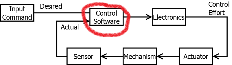
Again, for context, we are moving on to describe the contents of the software portion of our controller inside our standard control system:

Bang-Bang

Let us take a first pass at designing some software that takes in a speed command, and produces a voltage command, with the intent of getting our shooter wheel toward the commanded speed. Based on the known physical relationship between voltage and speed, we declare the following very simple control law:

1. If the speed is too low, send full power to the motor
2. If the speed is too high, send zero power to the motor.

In this case, “too low” implies “actual speed is less than desired speed”. “Too High” is just the opposite. Full power means 12V (since we are controlling voltage), and zero power means 0V. This leads to what is commonly called a “Bang-bang” controller - hopefully a pretty intuitive concept. Per its name, it causes the motor command to “bang” between max and min power, attempting to keep the speed right at the desired value. Hence the name, Bang-Bang Control.

Here’s an example of what such a controller would do:

Notice how at the beginning, the system keeps the motor on. As soon as the speed crosses the “desired” threshold of 1000RPM, the motor command drops off. The motor speed begins to decrease, and continues to do so until the speed falls below that 1000RPM bogey. Once it does, the voltage turns on again, full force. The motor speeds back up till it is turning the shooter wheel faster than 1000RPM. At which point the voltage shuts off, and the cycle starts over.

This control logic is actually remarkably good, especially given its simplicity (it’s an if/else statement). The only variable to really play with - how fast to you sample speed and update the output voltage? Usually this is fixed (~20ms on the roboRIO, unless you do something funky). Play with the slider above to see the effect - it should be somewhat intuitive. The faster you perform this update rate, the less “jerky” the motor speed gets. However, faster takes more processing power, and cycles the controller on and off faster.

The biggest disadvantage is that it’s causing big swings in the electrical signal, and slightly oscillating motor speed around the desired motor speed. If these voltage swings and slight velocity oscillations are acceptable for your application, this is a great system to use for controlling your shooter wheel.

However, there are more advanced options which can produce… “nicer” behavior.

PID Controller - What It Is

A common design that can work in lots of cases is the Proportional/Integral/Derivative controller, or “PID” for short. PID controllers are designed to take our previous “too-low/too-high” intuition, and use some mathematical operations to make it a bit more rigorous.

PID controllers output a single speed command which is the sum of a set of terms, each term scaled by the associated gain.

Error

A PID controller first computes the error between the desired and actual velocities:

$$\omega_{err}(t) = \omega_{des}(t) - \omega_{act}(t)$$

This error is then used in different ways in each term.

The PID Control Law

For the mathematically inclined, the PID control law dictates that the voltage shall be calculated according the the following formula:

$$v_{PID}(t) = K_{P} \omega_{err}(t) + K_{I} \int_{x=0}^{x=t}\omega_{err}(x)dx + K_{D} \frac{d\omega_{err}}{dt} + K_{F} \omega_{des}(t)$$

If this appears daunting, Fear not! We’ll break this down piece by piece.

Proportional Term - $K_{P} \omega_{err}(t)$

The proportional or P term uses the error $\omega_{err}(t)$, scaled by its gain $K_{P}$. This fundamentally accomplishes something very similar to what the bang-bang controller does.

When $\omega_{des} > \omega_{act}$, the P term is positive. When the opposite is true, the P term becomes negative.

When $\omega_{des}$ is very different than $\omega_{act}$, you get a large output from the P term. When the two are similar, the P term’s value is close to zero.

Assuming the signs in the system and $K_P$ are chosen well, our control effort output to the plant will generally move the plant in the correct direction.

This means, in a much smoother way, we emulate the behavior of the bang-bang controller, which intuitively should be moving you in the right direction.

Derivative Term $K_{D} \frac{d\omega_{err}}{dt}$

The derivative or D term uses the derivative of the error (with respect to time), scaled by its gain $K_{D}$. This adds some new functionality on top of the bang-bang controller.

Don’t get too scared by the usage of calculus here. The way to think about the D term is as a rate limiter on the P term. Think about if you were accelerating on the highway, but you see cars stopped way in front of you. You might continue to mash on the gas pedal, then hit the brake at the very last minute. You might also be insane if you do that. Sure, you could technically stop, but it’s way better to start slowing down before you get to your target.

That’s exactly what the D term is for - it helps make sure the “inertia” of the P term charging full force toward the goal is tempered a bit, and cuts back on our control effort in advance of us getting there.

This is useful for reducing overshoot, and slight oscillations of $\omega_{act}$ around $\omega_{des}$. We’ll discuss these in more detail later.

Integral Term $K_{I} \int_{x=0}^{x=t}\omega_{err}(x)dt$

The integral or I term again uses some calculus - this time, the integral of the error over time. Again, we’re adding new functionality beyond what our bang-bang controller could hope to do.

Again, don’t get too bogged down by the calculus. Think about what happens if you’re almost operating at the desired value, but not quite. $\omega_{act}$ will be very similar to $\omega_{des}$, but not exactly the same. As a result, your P term is very small - possibly small enough to not make much of a difference to the system’s behavior.

This is where the I term comes in. By adding up previous values of the error, we cause the I term to accumulate, and increase in value over time, as long as we’re not exactly on target (ie, $\omega_{act} = \omega_{des}$ exactly). This accumulation adds more and more influence to our sum overall, until the control effort is finally large enough to make a difference in the physical system’s state.

Feed-Forward Term $K_{F} \omega_{des}(t)$

For certain systems, it is useful to augment the PID logic with an additional term - the feed-forward or F term. Note that it uses $\omega_{des}(t)$, not $\omega_{err}(t)$. This means it has no dependance on your sensor feedback, only on the operator command.

The way to think about the F term is a “guess” at what $v(t)$ should be, prior to getting any sensor feedback or calculating any of the other terms. In general, for this shooter wheel, we know there is a linear relationship between steady-state speed and input voltage. That is to say, for a given input voltage, we know we’ll (eventually) settle out at some speed. With a bit of experimentation, we can even find that voltage that gets us to our (in these examples) 1000 RPM set-point. We take this information and “bake” it into our F term, which reduces the amount of “work” the other P, I, and D terms have to do to get the system behaving nicely.

The F term can be kind of tricky - if in doubt, leave it out. It works here because of the linear relationship between voltage and speed. If you were doing something like controlling an arm position with a motor, and trying to get the closed-loop system to achieve a certain arm position (not velocity), you’d definitely not want to use F like this. However for velocity control, like in shooter wheels, I think it’s almost impossible to live without!

Putting it All Together

And that’s all there is to it! Bask in the glory of the equation once more:

$$v_{PID}(t) = K_{P} \omega_{err}(t) + K_{I} \int_{x=0}^{x=t}\omega_{err}(x)dx + K_{D} \frac{d\omega_{err}}{dt} + K_{F} \omega_{des}(t)$$

The key to doing this is that you, as the engineer, have free control over picking $K_{F}$, $K_{P}$, $K_{I}$, and $K_{D}$, and just need to pick them to make your system act nicely.

Note that you may hear some people talk about a “PD” or “PI” controller - this is still a PID controller, just with the “missing” gain in the name set equal to zero.

Below is a sample of some nicely picked values. We’ll spend next time describing how to go about picking them. But for now, feel free to fiddle around with it, and refresh the page if you want to reset.

PID(F) Controller - Why it Works (or Doesn’t)

If you’re familiar with the math behind the PID controller, it’s not too hard to stare at it to convince yourself “Yea, this should probably work”. But, it definitely doesn’t work in all cases. In particular, it has to be tuned around certain system behavior. If that behavior changes drastically over the course of operation (mathematically a non-linear system), the PID system will often not perform as well. Things like slack in chains and gearboxes, static friction, squishy game pieces, and many other things will lead to systems becoming non-linear. In these cases, you can either:

1. Suck it up. Get it good enough, and walk away
2. Use a more advanced controller that accounts for the system’s non-linear behavior.

Similarly, the PID (especially the D term) are not good at handling noise in the system, and also make implicit assumptions about the amount of delay in the sensor feedback system. For this reason, make sure your sensors are good (ie - expensive and well-mounted). Also, be prepared to do additional work if using with a fundamentally high-latency system (like most vision processing has been, historically).

Conclusion

Sweet! We’ve covered the basics of what a controller is. In our 3rd and final installment, we’ll discuss how to tune a PID controller, and where to look for “next steps”. Check out the interactive post here!