Control Theory - Mathematical Models of the World

All models are wrong, but some are useful. - George Box

Introduction

This is Part 2 in our series on Control Theory. In this installation, we’ll look at how we describe the interior of the blocks in our block diagram, using math equations. By doing this, we will have a representation of functionality we can analyze, manipulate, and write software with.

What is a Model?

We briefly alluded to the concept of a model in Math Primer, part 2. A mathematical model is one particular form of an Abstraction, where we create math equations to describe the behavior of a particular thing in the “real world”.

Mathematical models can be built for anything which has properties you are willing to describe using numbers. This includes more conceptual things like a country’s economy or a stock market, but also physical devices (like motors or gearboxes or robots). We’ll be focusing on the latter.

If you’ve ever spent any time around a robot, you definitely have a qualitative model built up in your head of how lots of parts on the robot work. For example, you probably know that when you apply 12V to a motor, it starts to spin faster. Or if you reverse the wires, it will go the opposite direction. You might also know that if you put two different size gears together and turn one of them, the smaller one will be spinning faster and in the opposite direction of the big one.

These qualitative models are super useful - these are what we engineers use on a day to day basis to help understand the systems they work on, without the need for calculation. If you’ve ever seen an “old-timer” with a grey beard just magically come up with an answer to a robot design question, blurting out “That will never work!”, there’s a good chance that person was using a mental, qualitative model. Most people refer to these simply as “intuition” - with time working on devices, you start to get a feel for how they react and interact.

However, these models have limits. Often, a design may require you to describe how fast a shaft will turn. “Kinda fast” is a good starting point, but isn’t sufficient. You’ve hit the limit of the mental model, and have to go to the next level.

Here’s where the mathematical models come in. By doing some analysis, determining some equations, plugging in your operating conditions, and calculating an answer, you get the exact quantity you need for your design.

There is a key fact to keep in mind (as our friend George Box reminds us). Mathematical Models are more accurate than qualitative notions of how things work, but still do not fully describe the physical things we care about. And that’s ok, we don’t need a full description. Like any good abstraction, a mathematical model will hide the details we don’t care about, allowing us to focus on what we do care about.

For a concrete example, you will never see me construct a model for a motor that accounts for the magnetic fields of motors nearby. The “background” field strength is never large enough to make a difference in calculations of any quantity used for FRC. Qualitatively, I can tell you that if the background magnetic field was ever was big enough to matter, we have much more pressing issues on our hands than the couple percent error in our motor torque.

More detail is not always what you want. The right amount of detail is always what you want.

In this post, we’re going to briefly discuss how some models are built up, and quickly dive into a number of examples that will be useful for FRC.

Techniques for Building up a Model

First Principles

When we set out to create a model of a physical system, there are a couple different approaches.

The most “academic” approach involves analyzing the system from base physics principles. For FRC, $F=ma$, Maxwell’s equations, the Ideal Gas Law and friends come together with techniques like Free Body Diagrams, Differential Equations, and Linear Algebra to create a cohesive set of equations, accurately describing the quantities of interest. Or, at least, what they in theory should be.

Whether it’s ever explicitly shown, every mathematical model built up from base principles can be boiled back down into a set of axiomatic equations, based in how fundamental particles of the universe are assumed to interact. I’ll admit, I’ve never actually taken the time to take any of my models all the way back to these axioms. But I learned them once in college, and know (based on the techniques involved) I always could, if I ever needed to.

Soapbox: This is why, even if you find them pointless, all the foundational math and physics courses you take early on in your engineering education are very important. They lay the groundwork allowing you to prove that your calculations are correct later on. Study them hard, and trust they will be useful. Soapbox over.

Experimental Data

When base principles are hard or time consuming, and you have the ability to run experiments on the device in question, there is another approach available. You can gather data from your device under carefully controlled conditions to inform your model of how the device works. You make your model through pure observation. You have to run these experiments many times to ensure your results are consistent, and not being influenced by a factor beyond your control.

For complex devices, it is often faster to go the experimental route. However, these experimental models lack the detail about the “internals” of the system. There are few (if any) equations to re-arrange and re-solve for a particular quantity of interest - you’re kinda stuck with whatever you measured in the lab. Additionally, lacking details about the internals to the system, it’s harder to know how to redesign a particular device if it’s not working as you need. Though you’ve captured the “externally visible” behavior, you’re lacking insight about the inside.

Then again, you don’t always need that level of insight. It always depends.

Google & Datasheets

This isn’t exactly a “technique”, as much as something someone should keep in mind. Engineers are lazy. Engineers don’t like doing things twice.

However, if you as an engineer build a brand new device, you should probably take the time to take some measurements on it, maybe even build up a detailed model of how it should work.

Two bits of good news: Most engineers who are worth their salt will do experimentation. And, most of them make these experimental results available, in some form. Google is a great way to find out background info on whether someone has already done what you need to do - as long as you know what to search for. For example, look at the plethora of information available on describing motors!

The datasheet of a device is another standardized (ish) way of describing their quantitative properties. Sometimes a datasheet provides the exact mathematical model for the device. Other times, it provides the key pieces of information required for the model, and lets you build up the model as you need. Again, Google is my number-one tool for finding datasheets for parts we use. Manufacturers and suppliers frequently keep them on their websites as well.

The Need for Validation

No matter how you build up your model, you will always want to spend some time validating that it is producing meaningful results. Sometimes this means running experiments on the actual device. Other times, it means running your new model in some form of simulation - getting it into specific operating criteria, and checking results match some expected value.

Practical Example - Gearbox

Let’s start out with a model we can, for the most part, derive from the ground up.

A set of gears is probably one of the simplest models to create. It aligns well with your intuition, has a beautifully simple formula, and can be easily verified.

When designing gearboxes, you usually want to know about speed. Given an input speed (which you can control), you want to know what the output speed will be. Since many of you probably already know the answer, let’s just get that over with:

$$\omega_{out}(t) = -\frac{N_{in}}{N_{out}} \omega_{in}(t)$$

Where:

• $\omega_{in}(t)$ is the rotational speed of the input shaft at time $t$
• $N_{out}$ is the number of teeth on the output gear
• $N_{in}$ is the number of teeth on the input gear
• $\omega_{out}(t)$ is the rotational speed of the input shaft at time $t$

That’s it - it’s just the ratio of the teeth!

Spinning Levers

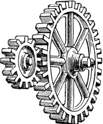
source: etc.usf.edu

The key thing to keep in mind: gears are just spinning levers. When you push on one, the other moves. The point at which the teeth mesh together is the fulcrum. Moving that mesh-point closer to the center of either wheel changes the ratio of motion between the two sides.

This relationship could be derived intuitively. Make the assumption that the teeth are always in mesh, and never slip relative to each other. Given this, it stands to reason that if there are 3x the number of teeth on the output, the input would have to rotate 3 times to get a single rotation on the output.

The logic flow for this: One tooth of motion on the input means one tooth of motion on the output. If you don’t have this 1 to 1 relationship, it means gears are slipping. Which means that metal is shredding off in your gearboxes. Which is bad news bears. You should fix that before attempting any more math.

A more rigorous way to describe this relationship is to do it from base principles and mathematical manipulations. Let’s give that a shot.

To start, assume that your teeth are “Ideal” - incredibly small, and super strong. They never slip relative to each other. We outright ignore any tooth geometry, and just model the gears as two differently-sized pancakes.

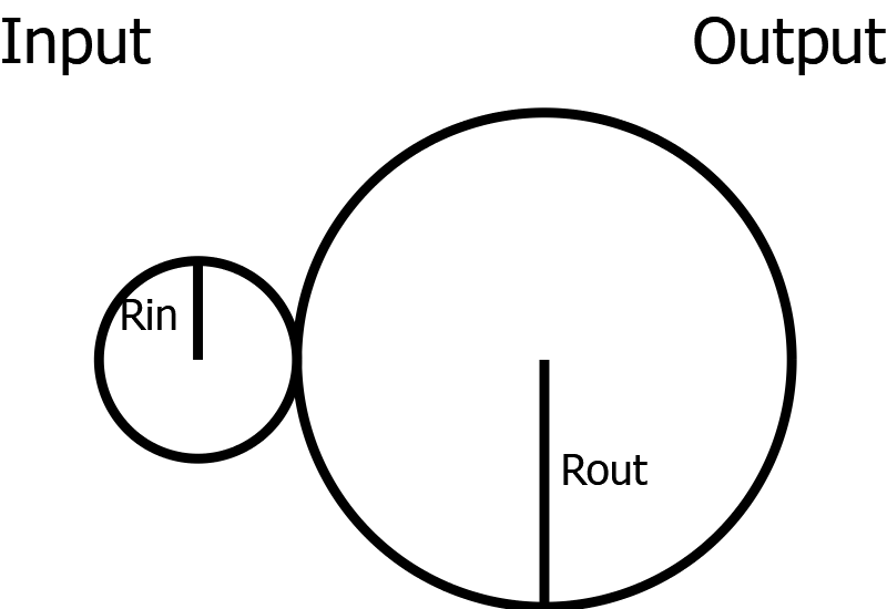
The assumption of ideal teeth allows us to say that the tangential velocity (the linear speed of the outside edge of the pancake) must be the same at their mesh point. From geometry, I’ll give the equation that relates the rotational velocity $\omega(t)$ to the tangential velocity $v(t)$. ¹

$$v(t) = 2 \pi R \omega(t)$$

We actually can write that equation twice, once for each gear:

$$v_{in}(t) = 2 \pi R_{in} \omega_{in}(t)$$ $$v_{out}(t) = 2 \pi R_{out} \omega_{out}(t)$$

Then, based on our ideal mesh assumption, we can set the two equal to each other. Note that since the tangential velocity is measured to the left of one center-point, but the right of the other, we need to introduce a negative sign as well. ²

$$v_{in}(t) = -v_{out}(t)$$ $$2 \pi R_{in} \omega_{in}(t) = -2 \pi R_{out} \omega_{out}(t)$$

Canceling terms, we find ourselves at:

$$R_{in} \omega_{in}(t) = -R_{out} \omega_{out}(t)$$

And solving for the output speed, finally,

$$\omega_{out}(t) = -\frac{R_{in}}{R_{out}} \omega_{in}(t)$$

Sweet! Almost the same as the equation we started with.

Radius to Teeth

But wait! Our initial equation used number of teeth, not radius. Not to worry!

Each tooth and gap cycle contributes a certain, constant amount of radius to the circle. Additionally, the per-tooth radius length has to be the same on both gears. This is due to some of the constraints required by good tooth design. Additionally, we aren’t actually free to choose any radius we want. If we resulted in a fractional tooth, well, that wouldn’t work (Think about it for a second…).

Therefor, the equation gets quoted not in terms of actual radius, but in terms of tooth count.

$$\omega_{out}(t) = -\frac{N_{in}}{N_{out}} \omega_{in}(t)$$

Boom Shackalacka.

On Torque

Torque is a concept that comes up a lot, isn’t something that most freshman start off knowing about, and frankly isn’t often explained well in physics classes.

I always think of torque is “turney force” - force that acts in a circle. Like when you turn a wrench, and tighten a bolt.

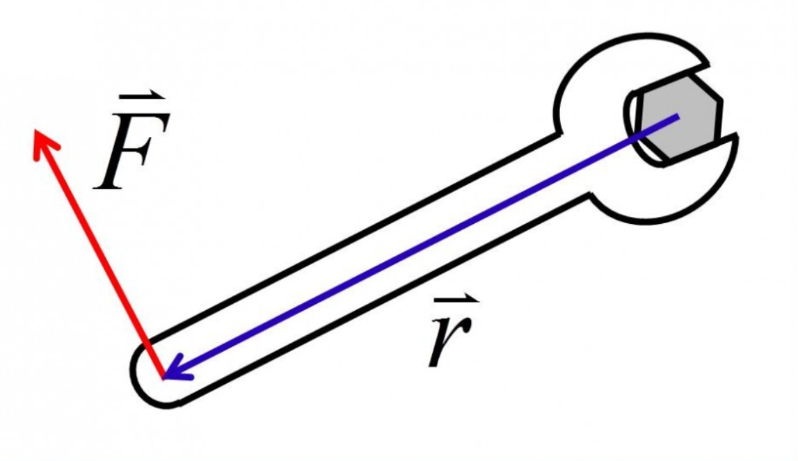
source: scienceres-edcp-educ.sites.olt.ubc.ca

Gears transmit torque from one to the other. We won’t get too much into the math, but it’s not hard to derive using the same lever-like models we eluded to before.

Torque in a gearbox is just a ratio, like speed, except inverted:

$$\tau_out(t) = -\frac{N_{out}}{N_{in}} \tau_in(t)$$

No need to worry about this too much now, but we’ll come back to it later on.

Practical Example - Wheel with Mass

Here, we’ll start to introduce the glory of using Google to find answers. The key is knowing what to look for.

We will attempt to create a model of a rotating wheel, such as the ones used to launch gamepieces through holes or into hoppers.

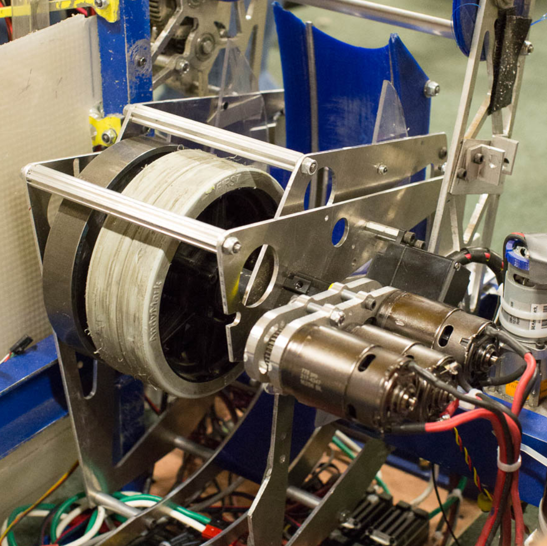
source: Team 1640

The key background info to know: Newton’s second law $F=ma$ has a rotational form.

Background - Newton’s Second Law

So, hopefully, you’ve at least heard the basics of Newton’s laws in school. They form the basis of “classical mechanics” - the study of how bodies of mass move around (as long as they aren’t too small, and don’t move too fast). The second law is the one most commonly quoted in its equation form, but can be understood qualitatively. Whenever a force $F$ is applied to some object with mass $m$, it will begin to change velocity at a rate $a$. Forces are how we change the velocity of an object.

It should be noted that $F$ and $a$ are usually vector quantities. That is to say they have both magnitude and a direction. You can push with 5 lbs of force upward or downward, to the left or to the right. The magnitude is always 5 lbs, but the direction changes. To denote this vector quantity, you will often see the equation written as

$$\vec{F} = m\vec{a}$$

The cute little arrows over $\vec{F}$ and $\vec{a}$ indicate they have a direction.

The key takeaway is that the acceleration happens in the same direction as the force. If an object is still, and you push on it in a certain direction, it begins to accelerate (ie, go faster) in that direction. If an object is already moving, and you push against its motion, it slows down, since the force opposes the direction of motion - effectively a negative acceleration.

Newton’s Second in Rotational

To me, the rotational form of $F=ma$ almost feels like cheating. The good news is that it makes it pretty simple, but perhaps not profound. The reason for this is that all three quantities in $F=ma$ have a rotational equivalent we can use.

If you hadn’t noticed yet, $F$ and $a$ are both quantities that involve linear measurement. This is the nature of vectors - they define lines from one point to another. Acceleration is described along a certain line, as is force.

On the other hand, mass tends to just kinda “sit there” - it’s a property of the object, with a value, but no real direction or information about location required. As far as Newton’s Second law is concerned, all the mass is modeled to be at a single point, where force is applied.³

Newton’s Second Law for rotation is exactly the same as the linear version, just swapping out the linear quantities for their rotational equivalent.

Acceleration is easy to re-define - it’s just called rotational acceleration. Rather than measuring the rate of change of linear velocity (in m/s, per sec, for example), it measures the rate of change of rotational velocity (in deg/sec, per sec, for example). Think of it as the rate at which a rotating wheel speeds up or slows down. If you want your wheel to rotate faster, that means you want its rotational acceleration to be positive.

Rotational Acceleration is denoted with the Greek letter alpha - $\alpha$

Force also has a rotational analog. Torque is simply rotational force. Torque is defined as a force applied at a distance to some center of rotation, tending to cause rotational motion. Whenever you turn a wrench or a screwdriver, you are applying a torque to the bolt or screw, which causes it to turn. Whenever your car’s engine revs up while you’re in gear, a torque is applied to the back wheels (often erroneously referred to as “torque to the ground”). This in turn causes the wheels to turn, and (hopefully) the car to move.

Torque is denoted with the Greek letter tau - $\tau$.

Mass, turns out, is where things get a bit interesting. No longer can we simply account for the total amount of stuff in the moving object, we have to account for where it is at relative to the center of rotation. This combined notion of quantity and position can still be calculated down to a single number, called the moment of inertia.

Just as mass can be thought of as “tendency of an object to resist changes in velocity”, the moment of inertia is an object’s tendency to resist changes in rotational velocity.

The way I personally like to think about it - consider the energy of tiny subsections of our spinning object. At any given rotational velocity, all will have the same rotational velocity. However, the bits near the center will have less linear velocity. They’ll be traveling slower, at least in a linear sense. This means they have less energy, and would hurt less if they hit you. If you want to change the speed of a rotating bit of mass, it’s easier if the rotating bit is very close to center of rotation, rather than really far away.

These moments of inertia still boil down to a single number, and are usually calculated with integrals. Deriving them from scratch is a classic calc-II homework problem. You should definitely try it at some point in your life.

However, I’ve already passed all my calculus courses, so I just look them up online..

Since $M$ can mean things like “mass” or “mega” or “million”, Moment of Inertia is indicated with the letter $I$. Even though $I$ is also used for electric current. I’m sorry, I didn’t make any of this up. There aren’t many letters available. Usually it’s clear from the context of the equation which is meant…

Assembling the Equations

Ok, starting with Moment of Inertia…

Partway down the table, you’ll see an equation for “Solid cylinder of radius r”.

source: wikipedia.org

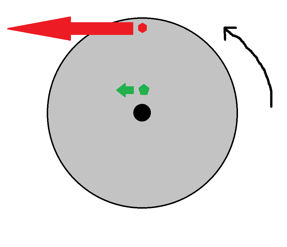
Recalling that we’re attempting to create a model of a shooter wheel, this should look pretty familiar. Think wheel on a stick, rotated around the axis of the cylinder-shape (Z axis in the wikipedia picture). Wikipedia tells us the equation to use is:

$$I = \frac{1}{2}mr^{2}$$

To quickly break this down:

$m$ is the mass of the whole shooter wheel $r$ is its radius

We assume that the mass is reasonably evenly distributed throughout the whole radius. For something like a colson wheel, this is likely true. If you have something more like a Plaction Wheel, you might want to pick a different equation.

Now, we can substitute all the variables into Newton’s Second Law for Rotational Motion:

$$\tau(t) = I \alpha(t)$$ $$\tau(t) = \left( \frac{1}{2}mr^{2} \right) \alpha(t)$$ $$\alpha(t) = \frac{2}{mr^{2}} \tau(t)$$

And there we have it! A simple description of the motion of our shooter wheel, given a certain torque (or “turney force”) at its input shaft! This is the equation we’ll need later on.

As a quick detour, let’s throw in a bit of calculus. We can describe the wheel’s velocity over time as an integral.

In general, we know that velocity $\omega(t)$ is the integral of acceleration $\alpha(t)$:

$$\omega(t) = \int \alpha(t)$$

Applying more proper calculus and our previous equation:

$$\omega(t) = \int_{0}^{t} \frac{2}{mr^{2}} \tau(x) dx + \omega(0)$$

In general, we can assume $\omega(0)$ is in fact 0, since our robot starts the match from a disabled state.

$$\omega(t) = \int_{0}^{t} \frac{2}{mr^{2}} \tau(x) dx$$

What this equation shows is is that to know the velocity of our shooter wheel, all we have to do is add up all the previous torque inputs we ever gave to it, multiply each measurement by the moment of inertia (just a constant number, tied to the wheel’s construction), and Bob’s your uncle! We’ve come up with an equation that calculates the shooter speed over time, as a function of how much torque you apply to it.

Ok, detour over. Hope you enjoyed Calculusland!

Practical Example - Brushed DC Motor

Basic Description

A motor, fundamentally, is a device which converts electrical power into mechanical power. Specifically for our analysis, we’ll look at it as a device which takes an input voltage and current and produces a mechanical torque on its output shaft. Presumably this is attached to something which maybe fights against the rotation, but ultimately rotates. This speed of the input shaft “feeds bacK” to the motor as another input.

The key thing to realize - the motor doesn’t directly output rotation. It outputs a torque - a force on something attached to it. Rotation only occurs if the thing attached to it starts to rotate in response to that torque.

We’ll be analyzing brushed DC Motors. This covers CIM motors, 775 pro, and pretty much every FRC motor used up till NEO’s in 2019 (sorry Rev). Though they come in different sizes, shapes, weights, and powers, they all fundamentally act the same way:

Electric current flows through coils of wire, generating a magnetic field. Trust me, it happens. The coils are mounted on a rotating shaft, aligned within a set of permanent magnets, so that the generated magnetic field from the coils opposes that of the permanent magnets. This opposing field causes a force on the rotating shaft, which is transferred to the motor’s output shaft. A special electromechanical device called a commutator ensures that the coil’s magnetic field always opposes the magnet’s fields, throughout the whole range of rotation.

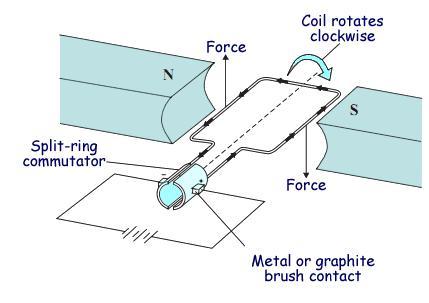
source: mouser.com

Torque

The first key takeaway from our description: a flowing electric current is the cause of the force on the output shaft. This leads to the first part of the equation for motors:

$$\tau(t) = K_T I(t)$$

Where:

$I(t)$ is the current flowing through the motor at time $t$

$K_T$ is a constant value, called the “Torque Constant”.

$\tau(t)$ is the torque at the output shaft of the motor at time $t$

The Torque Constant $K_T$ is something you could try to calculate from the geometry of the motor, the properties of the coils of wire, the strength and shape of the magnets, and a whole slew of other properties. If you were to do all the physics and math you’d be able to generate the relationship seen above, with a very complex and inaccurate version of $K_T$. For most motors, it is determined experimentally.

Most motors should list it in their datasheet, at least indirectly. If you don’t see anything labeled $K_T$ or “Torque constant”, you can also just quickly calculate it from the stall conditions of the motor. Stall conditions provide one particular $\tau(t)$ and $I(t)$ pair to use:

$$K_T = \frac{\tau(t)}{I(t)} = \frac{\tau_{stall}}{I_{stall}}$$

Speed

The shaft speed impact is a bit harder to think through, but not too bad.

You may have heard at some point in your life that all motors can act as generators, and all generators can act as motors. Even if you haven’t heard this, maybe you’ve seen your robot electronics power on when you push your robot along the ground, even without a battery in it? You’re not going crazy, your motors are acting as generators and powering the system!

Though the equivalency expressed above is largely true, I prefer a slightly different twist: every motor is simultaneously a motor and generator. This simultaneous existence should make sense - there’s nothing that physically changes about a motor when you rotate its shaft, versus when you power it electrically. It doesn’t magically know when it needs to switch modes. Both modes must be present at all times.

You’ve probably also noticed that when you plug in a motor straight to 12V ⁴, it will zoom up to some top speed, stop accelerating, and maintain that top speed. Datasheets call this the “unloaded” or “runout” speed.

But wait! If there’s current flowing, that means there should be torque, right? Which means there should be acceleration?

In a sense, torque is the “Motor” part of the “simultaneous motor and generator”. The generator half explains the capped speed.

Whenever you have coils of wire rotating within a magnetic field, a voltage is formed across the coil. Voltages, when present in well-behaved circuits, will increase or decrease current flow. This is how generators work - spin a coil of wire near permanent magnets,a voltage is created, which enables current to flow out.

Hey wait. Motors have coils of wires spinning in a magnetic field. Yup. There’s no trick here - the fact that the wires are spinning within the magnets inside motors causes a new voltage to be induced within the wires, which actually opposes the flow of current. This induced voltage is called “Back EMF”, or “Back ElectroMotive Force”.

Very similarly to torque (as you would hopefully expect from all the symmetry we’ve seen so far), this back EMF is linearly related to speed:

$$v_{emf}(t) = K_V \omega(t)$$

This back-force happens in the electrical space, so it’s good for us to look at an electrical model of the motor:

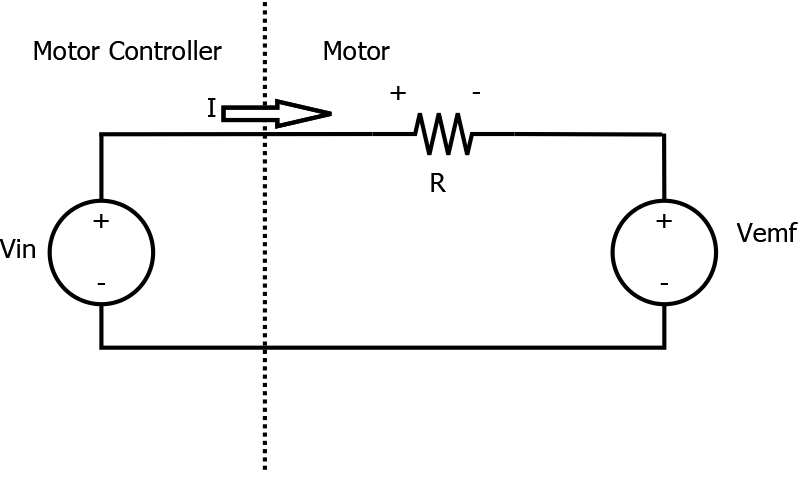
On the left side, we see the input wires to the motor, along with two measurements you may already be familiar with. One is the applied voltage $V_{in}(t)$ - this is the command you give to a motor controller, and the average voltage it outputs to the motor. Usually this will be about +12V for full forward, -12V for full reverse, and 0V at rest (though the numbers usually change with battery charge level). The other quantity is the current flowing through the motor, $I(t)$. This might be measured by a motor controller (if you have a nice Talon SRX or similar), or measured by the PDB itself. Either way, you usually don’t directly control it, it’s just a property of the current state of the whole system.

You’ll notice two things to the right, on the “inside” of the motor. One is a resistor - this electrical component models the resistance of the long coils of wire inside the motor. It’s not literally a resistor component inside the motor, just the inherent resistance from having lots of wire. Some models also include an inductor to model the “cross-talk” between the coils, but I’ve avoided it to make the calculations simpler. Often, it’s small enough you can forget about it.

Finally, the voltage source to the far right indicates the back EMF, which we denote with $V_{emf}(t)$. Even though the physical mechanism looks very different, the electrical effect is the same as the voltage provided by your motor controller.

When analyzing a circuit diagram like the one above, we use Kirchhoff’s Circuit Laws to construct equations. The laws give us a few facts:

• The current through every device must be the same.
• The sum of voltages around the (one and only) loop must equal zero.

Since $V_{in}$ is oriented backward relative to the +/- direction defined for the other components, it gets a minus sign.

$$0 = -V_{in}(t) + V_R(t) + V_{emf}(t)$$ $$V_{in}(t) = V_R(t) + V_{emf}(t)$$

If you recall Ohm’s Law from the electronics introduction, you’ll see we can re-write the voltage across the resistor ($V_R$) in terms of the motor current and the resistance. Additionally, as shown before, the back EMF voltage can be calculated from the speed of the motor.

$$V_{in}(t) = R I(t) + K_V \omega(t)$$

Solving for current:

$$I(t) = \frac{1}{R} \left( V_{in}(t) - K_V \omega(t) \right)$$

Finally, we can use our current/torque relationship to solve for torque:

$$\frac{1}{K_T} \tau(t) = \frac{1}{R} \left( V_{in}(t) - K_V \omega(t) \right)$$ $$\tau(t) = \frac{K_T}{R} \left( V_{in}(t) - K_V \omega(t) \right)$$

Practical Example - Wheeled Shooter System

Alright. It’s time to combine our equations together. Here’s what we’re looking to describe: We want create an equation for speed of our shooter wheel, given the applied voltage.

The basic process - the applied voltage in the motor produce a torque. This torque is transferred through a set of gears with a particular ratio. This torque acts on the spinning mass, causing an acceleration. Integrating that acceleration over time produces the speed.

Building the Full Equation

Starting from our most recent equation, we can calculate the output torque of the motor:

$$\tau_{motor}(t) = \frac{K_T}{R} \left( V_{in}(t) - K_V \omega_{motor}(t) \right)$$

The motor torque is the input to the gearbox. We know we can also calculate the output torque of the gearbox:

$$\tau_{wheel}(t) = \frac{N_{out}}{N_{in}} \frac{K_T}{R} \left( V_{in}(t) - K_V \omega_{motor}(t) \right)$$

And, given the torque at the output of the gearbox (which is the same as is applied to the shooter wheel), we can calculate the acceleration of the shooter wheel:

$$\alpha_{wheel}(t)= \frac{2}{mr^{2}} \left( \frac{N_{out}}{N_{in}} \frac{K_T}{R} \left( V_{in}(t) - K_V \omega_{motor}(t) \right) \right)$$

And, we can use the gearbox ratio to get the $\omega(t)$’s are in terms of the shooter wheel speed:

$$\alpha_{wheel}(t) = \frac{2}{mr^{2}} \left( \frac{N_{out}}{N_{in}} \frac{K_T}{R} \left( V_{in}(t) - K_V \frac{N_{in}}{N_{out}} \omega_{wheel}(t) \right) \right)$$

And finally, we combine constants to make stuff a bit easier to read (hopefully):

$$\alpha_{wheel}(t) = \frac{2N_{out}K_T}{mr^{2}N_{in}R} V_{in}(t) - \frac{2K_VK_T}{mr^{2}R} \omega_{wheel}(t)$$

Actually, this isn’t all that bad. Really, we have something like this:

$$\alpha_{wheel}(t) = C_1 V_{in}(t) - C_2 \omega_{wheel}(t)$$

With

$$C_1 = \frac{2N_{out}K_T}{mr^{2}N_{in}R}$$ $$C_2 = \frac{2K_VK_T}{mr^{2}R}$$

Both of which are just constant values (ie, numbers) related to the physical parameters of the system. Calculate them once, never think about it again. Nothing scary - just numbers.

The scary part to me - we’ve got a differential equation. That’s right - remember how acceleration is the derivative of velocity? $\alpha(t)$ and $\omega(t)$ aren’t just two random, independent values. Our equation really is:

$$\frac{d\omega_{wheel}}{dt} = C_1 V_{in}(t) - C_2 \omega_{wheel}(t)$$

Which, indeed, is an equation which involves a function $\omega(t)$ and its derivative $\frac{d\omega}{dt}$. This makes it a differential equation.

Tackling the Differential Equation

The good news - this is a very special type of differential equation - It’s called a “First Order, Ordinary Differential Equation” which, as it turns out, has a well defined analytical solution. Any college engineering program worth its salt will spend at least one semester teaching you about this.

There’s a different way I prefer to introduce high schoolers to how to solve this, though. Let’s cheat a bit, and pretend we’re software. Software isn’t looking at the speed at every time $t$, in some continuous fashion. Instead, it is sampling values at regular intervals. The length of the interval is called the “sample time”, indicated by $T_s$. It is usually around 20ms on the roboRIO, or 1ms on a talon SRX.

Let us quickly define some new nomenclature - when we describe some function that changes over time, we usually write it as $\omega(t)$, where the $(t)$ indicates that $\omega$ is in fact a function defined for every floating-point value time $t$. There’s another way of representing functions that indicates they are only really defined at regularly-sampled intervals, with the intervals counted by some integer $n$. The parenthesis are replaced with square brackets to indicate the sampled nature of the function, rather than a continuous definition.

So, if we wanted to represent how software sees this function, we write down $\omega[n]$, where integer $n$ is in the range $0, 1, 2, 3, ...$, and indicates the loop iteration of software. For any given sample time $T_s$, we can always know that $t = T_sn$

The key reason to do this - in discrete time, derivatives become very easy to do - they’re just subtraction:

$$\frac{d\omega}{dt} \Rightarrow \frac{(\omega[n] - \omega[n-1])}{T_s}$$

This should make a decent amount of sense if you stare at it. Remember that derivatives are like the slope of a graph of the function, and slope is rise over run, or $dy$ over $dx$. This is exactly what we have here - the change in $\omega$ divided by the change in time.

Switching our equation to be discrete-time (“software view”), and substituting in the derivative:

$$\frac{(\omega_{wheel}[n] - \omega_{wheel}[n-1])}{T_s}= C_1 V_{in}[n] - C_2 \omega_{wheel}[n]$$

And re-arranging:

$$(\omega_{wheel}[n] + T_s C_2 \omega_{wheel}[n] )= T_s C_1 V_{in}[n] + \omega_{wheel}[n-1]$$ $$\omega_{wheel}[n] ( 1 + T_s C_2 )= T_s C_1 V_{in}[n] + \omega_{wheel}[n-1]$$ $$\omega_{wheel}[n] = \frac{T_s C_1 V_{in}[n] + \omega_{wheel}[n-1]}{( 1 + T_s C_2 )}$$

And there we have it! An equation for the present speed of the shooter wheel, in terms of things we know:

• The speed calculated from the previous loop - $\omega_{wheel}[n-1]$
• The voltage getting applied to the motor this loop - $V_{in}[n]$
• Constants related to our physical system and software design - $C_1$, $C_2$, and $T_s$.

Whoof. There we go. As my dog would say, that was ruff. But we’ve made it. We’ve arrived. We have our equation.

Non-time-domain Analysis Methods

Ok. So to levelset - so far, we’ve been using what controls engineers would call “Time Domain” analysis. This all means that our equations have time as the independent variable. Whether we represent it as a continuously changing quantity $(t)$ or a discretely sampled value $[n]$, we use time as our variable that marches along, and that we analyze behavior across.

Time domain is intuitive. You can very easily think about how how physical quantities (like speed or voltage) change over time.

However, this is not usually how controls engineers work. The reason is the same one we ran into right at the end - differential equations. These are notoriously difficult to solve and work with in the time domain.

As it turns out, or friends from pure mathematical fields have devised a whole slew of other tools to use. You don’t have to use time as your independent variable - you can in fact use something else. Frequency, or a complex number representing frequency-like information, is the more common choice. Just like our quantization assumption, these frequency-domain analysis techniques convert the difficult task of differentiation and integration into simpler tasks like multiplication and division.

These transforms are not trivial concepts to cover, so I am calling them out of scope for now. If you’re interested in digging into these topics, the terminology to look up is Fourier Transform, S transform, and Z transform. These topics are also covered in the Control Systems in FRC textbook.

On Units

One piece of advice I would offer while working on these models - units will kill you. You will want to be super careful and rigorous in ensuring all your math and your constants are using the same units, and when you write your code, the units assumptions come in as well. We’ve kinda skirted the whole topic so far, as to not clutter the explanation. Still though, you have to be careful.

Honestly, I’ve only ever had success making these models using metric units, and being super-consistent on what prefixes I choose for each value. I do all the internal math and constants calculations in metric. Imperial has too many “gotchas” for me on the conversions.

However, I’m from the US. I grew up using feet and lbs, and I still have a far more intuitive understanding of what “10 feet per second” or “15 foot pounds of torque” looks and feels like - much more so that “15 meters per second” or “20 Newtons”. For this reason, any time we report values to a dashboard or log them to file, we convert back to imperial. It’s totally computational overhead, but I’d prefer to let the processor do that heavy lifting, and have a feeling for what the numbers mean, rather than waste my time doing mental math to do the conversion.

At the end of the day though, what matters most is that you produce a functional robot, and can tune and change things on it quickly. However you can best accomplish this is the right path for your team.

Conclusion

I feel as though we’ve come a very long way, but we also still have quite a ways to go yet! Hopefully you’ve enjoyed this worked-example of creating a mathematical model for a shooter wheel. Next up, we’re going to try injecting a few input voltages to our system to see how it reacts, and decide what sort of strategies work well to control the system to a commanded speed. Check out Controller Design for more info!